
Tutorial 2: Using the NeuriteQuant wizard
This tutorial provides step-by-step instructions to define analysis settings for NeuriteQuant using the wizard-type optimization procedure.
Before going through this tutorial, make sure to go follow tutorial 1 first.
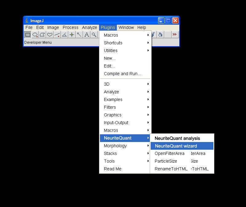
Open ImageJ, make sure, that no images or results are open, and choose Plugins, NeuriteQuant, NeuriteQuant wizard
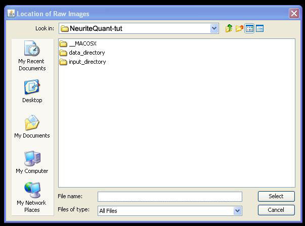
You will get a message that unsaved results will be lost by running the wizard. If you wish to continue, click 'Yes'. You will then be prompted to point to the directory, in which your raw images are stored. Point to the "data_directory" sub-directory from the tutorial data (see tutorial 1).
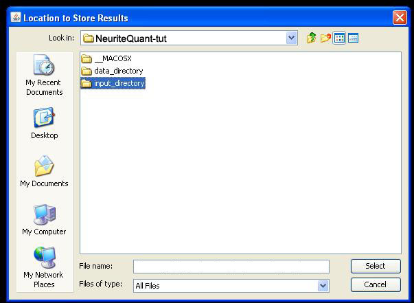
Next, you will be asked to point to the directory, in which your results should be stored. Point to the "input_data" sub-directory from the tutorial data (see tutorial 1).
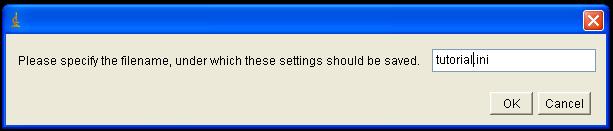
You will then be prompted to provide a filename, in which the analysis settings will be saved. For this test run, type in tutorial.ini.
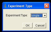
You will now need to choose which type of experiment you would like to perform. For this tutorial, we will perform a 'simple' experiment, in which only one experimental unit (such as 1 plate, for example) will be processed. Choose 'single' as the Experiment Type.
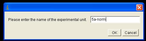
You will be asked to provide the name of the experimental unit. Depending on the imaging device used, and the way how images are stored by that device, this could be a folder in which images are saved, or a barcode, which is part of the image filenames, etc. For this tutorial, images produced via a custom script for the software Metamorph contain the barcode 5a-norm. Thus, the experimental unit for this tutorial is '5a-norm'.
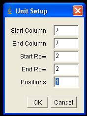
You will be asked to enter, which parts of the experimental unit should be analyzed. Experimental units are usually organized into rows, columns and positions. The tutorial dataset contains a subset of data from a 384-well plate. For this tutorial, enter the following values:
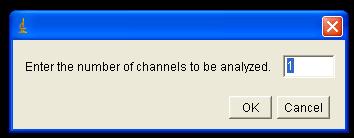
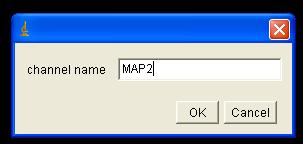
You will need to enter how many channels (staining colors) you wish to analyze. The dataset contains 3 channels. For simplicity, choose 1. You will then be asked to name that channel. Type in MAP2 as the channel name.
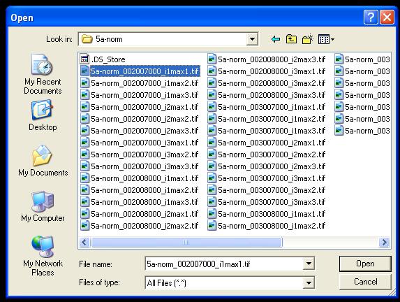
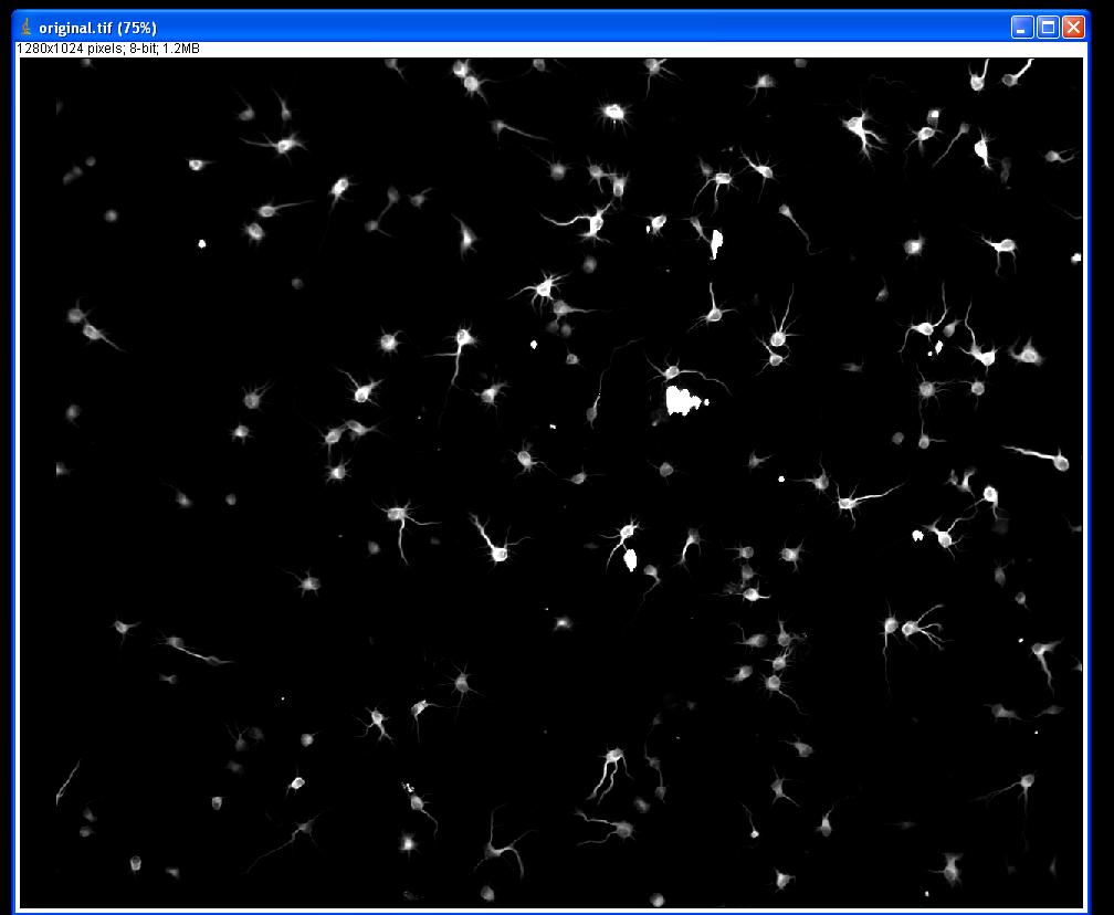
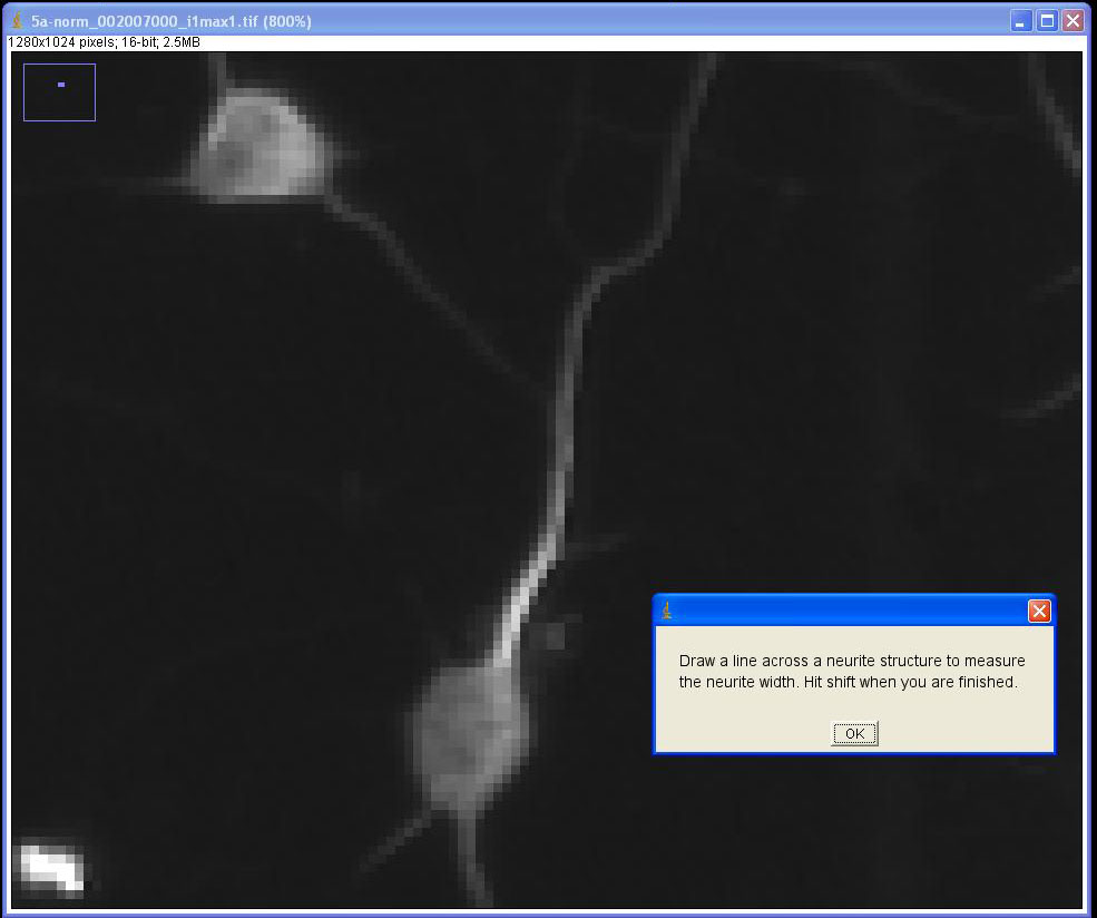
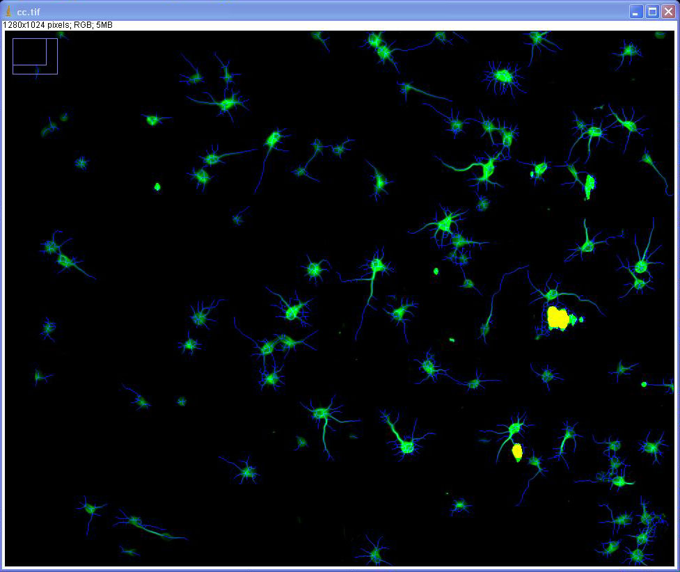
You now have the choice, whether or not to perform a wizard-type optimization to find suitable analysis parameters. This option is best if you are not yet familiar with NeuriteQuant. Choose 'Yes'. A pop-up window will prompt you to open a representative image file, which contains the maximal neurite density you wish to be able to quantify. Confirm this message by clicking 'OK'. Then, in ImageJ, choose File, Open File and then open the file indicated below (located in the directory: .../NeuriteQuant-tut/input_directory/5a-norm/):
The image opens and is displayed on the screen:
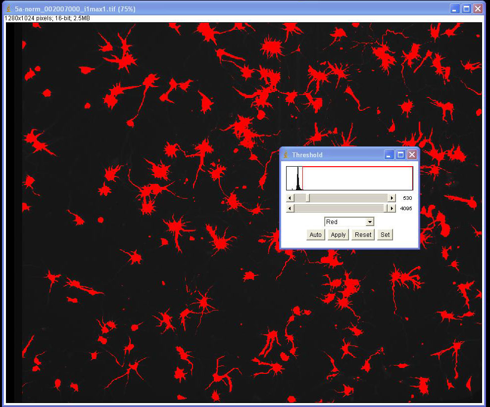
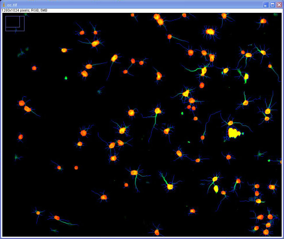
press shift to continue. A message appears to introduce the thresholding procedure. Confirm by clicking 'OK' an then move the upper slider in the threshold window until all neurons are nicely masked by the red threshold color (note that the algorithm performs a more sophisticated thresholding procedure for detecting neurites). Try to be all inclusive at this stage and make sure that all neurite structures, even the dimmer ones, are included in the threshold, i.e. are red). For this tutorial, set the threshold to 530 as indicated below. Press shift to continue. You now get another message to explain the use of the lower slider. Confirm by clicking 'OK'. Please note that the current image is saturated and thus the slider does not need to be moved further to the right for optimal results. Press shift to continue.
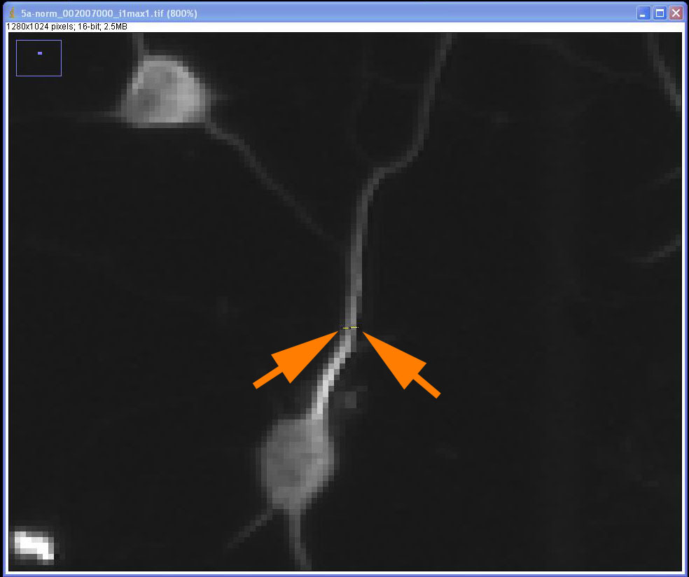
You will now need to zoom into a typical neurite area to define the neurite thickness. Confirm the message by clicking 'OK' and then click several times on the image into a region, into which you wish to zoom. Aim for a zoom of about 800%. Press shift to continue.
You will now need to draw a line across the neurite width. Confirm the message by clicking 'OK' and then click at the neurite and drag the mouse across the neurite width as indicated below. Press shift to continue.
You will get a message explaining the procedure. Confirm it by clicking 'OK'. You will also need to enter the first set of settings (neurite detection threshold, neurite cleanup threshold and neuronal cellbody detection threshold). Keep the default settings for all these parameters and confirm each entry box by clicking 'OK'. After confirming the last entry box, the algorithm will start analysis. Do not disturb the procedure by clicking any windows during this time. After analysis finished, you will get a representation of the analysis:
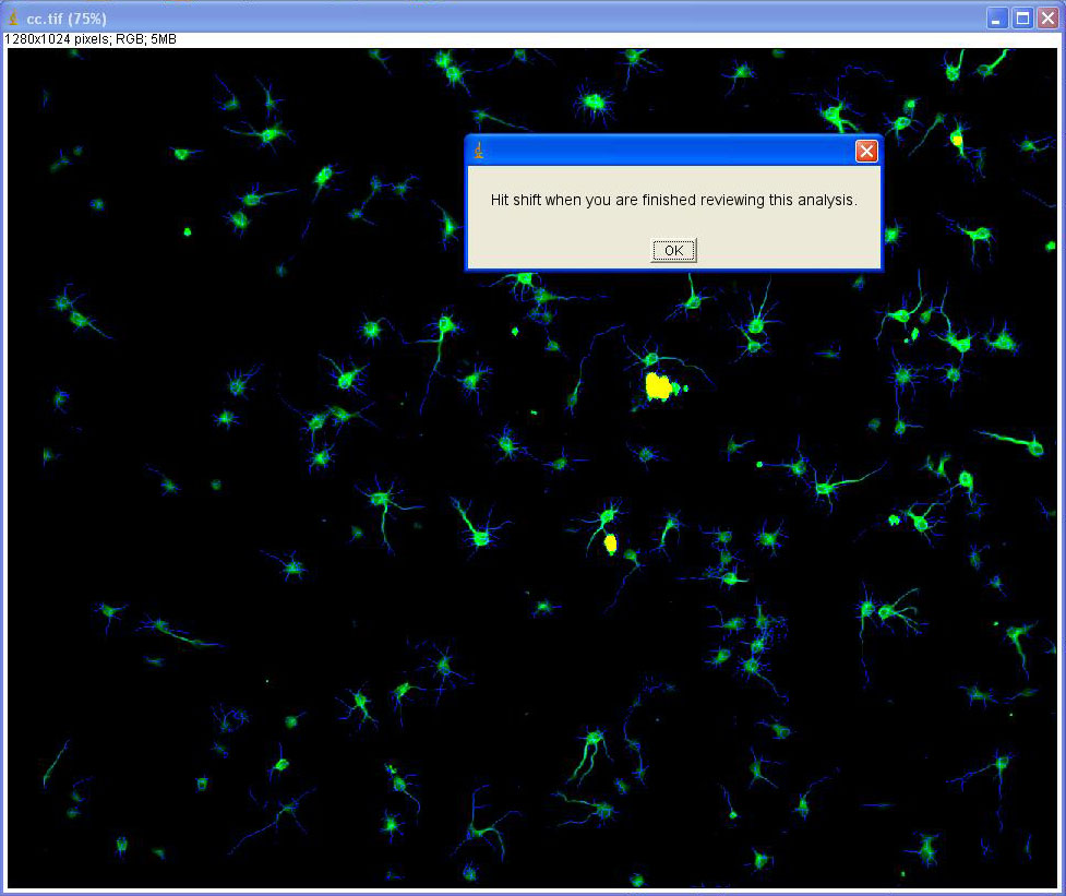
Confirm the message by clicking 'OK', review the analysis trace. Note, that the blue lines represent the neurite measurements and red blobs represent neuronal cellbody measurements. At this stage, the neurite analysis is still fairly coarse and the cell body analysis is not yet performed. Let's continue and use a higher sensitivity for detecting the neurite. Hit shift to continue. You will now be asked, whether you wish to test another set of parameters. Confirm by clicking 'Yes'. Choose 'No' when prompted if you also wish to adjust the scaling of the image. Now, change the value for neurite detection threshold from 5 to 2. Leave the default values for the other parameters untouched. After analysis is finished, confirm the message by clicking 'OK' and review the analysis trace. With the higher sensitivity, a few additional neurite structures will be detected. However, depending on the amount of background or the other analysis parameters, lower sensitivities might have lower variability and might give more consistent results. Note that there are also several small 'fragments' of neurite traces, which often just belong to background signals. Let's set the parameters to remove these. Hit shift to continue. Confirm to test another set of threshold parameters. Keep the value for neurite detection threshold at 2, change the neurite cleanup threshold to 50 and leave the value for neuronal cellbody detection threshold at 255. After analysis is finished, confirm the message by clicking 'OK' and review the analysis trace. Smaller neurite fragments have been removed. Higher values in the neurite cleanup threshold will remove increasingly larger neurite fragments from the analysis. However, if you use the standard zoom setting of 75%, note that some neurite tracings appear to be interrupted. Make sure to zoom to 100% to better evaluate the neurite tracing. Do this via ImageJ by clicking on Image, Zoom, View 100%:
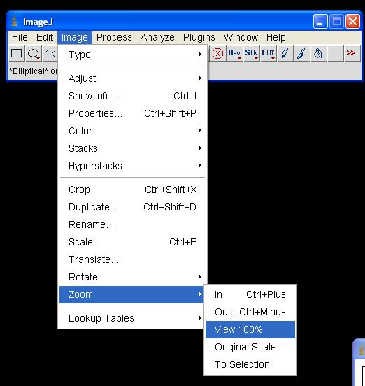
You will now be able to carefully evaluate the neurite trace analysis. Artifactual interruptions in the neurite tracing will be fixed at a zoom level of 100%.
The neurite traces are now of acceptable quality. Let's move on to detect the neuronal cell bodies. Hit shift to continue. Confirm to test another set of threshold parameters. Keep the value for neurite detection threshold at 2, keep the neurite cleanup threshold at 50 and change the value for neuronal cellbody detection threshold from 255 to 100. After analysis is finished, confirm the message by clicking 'OK' and review the analysis. Note that some but not all neuronal cellbodies were detected and displayed as red blobs. Repeat the procedure and change the neuronal cellbody detection threshold from 100 to 25. Now, most cellbodies are detected. Note that, depending on the background levels and other analysis parameters, a high sensitivity in the neuronal cell body threshold might lead to high variability. A lower sensitivity, at which very weakly stained cellbodies are excluded from analysis, might yield more consistent results. Now that all settings are optimal, continue by pressing the shift key and then choose 'No', when asked whether you wish to test another set of parameters.
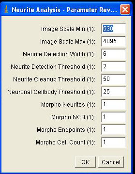
The program will now ask you a series of questions to determine which parameters should be measured in the analysis. Click 'Yes' for all parameters. NeuriteQuant will then present a dialog box in which the parameters identified by the wizard can be reviewed and changed if necessary. Note: if you chose not to use the wizard-type optimization procedure, you are directly transferred to this step to manually enter the parameters of your choice.
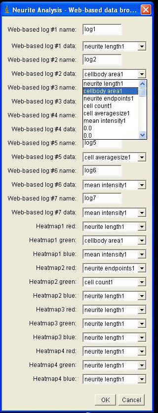
Finally, you can set which parameters should be presented in the web-based data-browser. Here you can choose which measurement parameters should be reported in the web-based log, and which parameters should be used to generate the heatmaps. Note, that the X-Y plots that are generated in parallel use the red and green values from the heatmaps as X- and Y-Axis parameters. Choose the settings you would like to use for the web based data browser and confirm by clicking 'OK'.
Now the settings file is saved into the input_directory (named tutorial.ini, as requested). You can now run the analysis by following the steps in tutorial 1, except, that you need to choose the tutorial.ini file you just generated, instead of the default test_set.ini file.